Shinyscholar

A template for creating reproducible Shiny applications

Simon Smart

June 7, 2025

Overview

Use of Shiny in academia
How Shinyscholar helps to avoid common problems
How to use create_template() to make an app
How to develop modules

Please ask questions!

About me

Background in plant sciences and agricultural science
Software developer in the Department of Population Health Sciences at the University of Leicester with Tim Lucas
Latecomer to R, starting in 2018
Quickly fell in love with Shiny

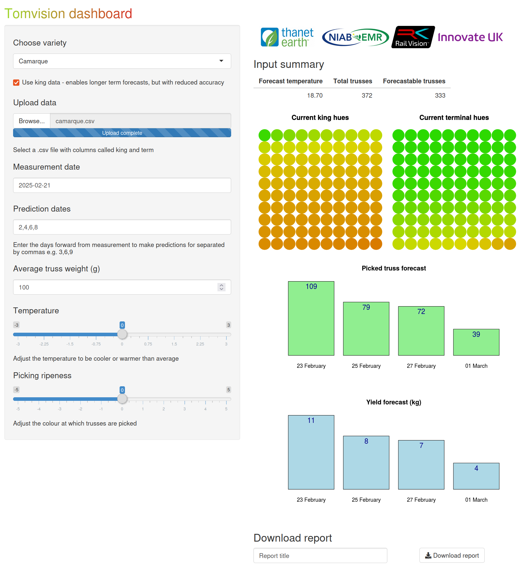
Tomvision

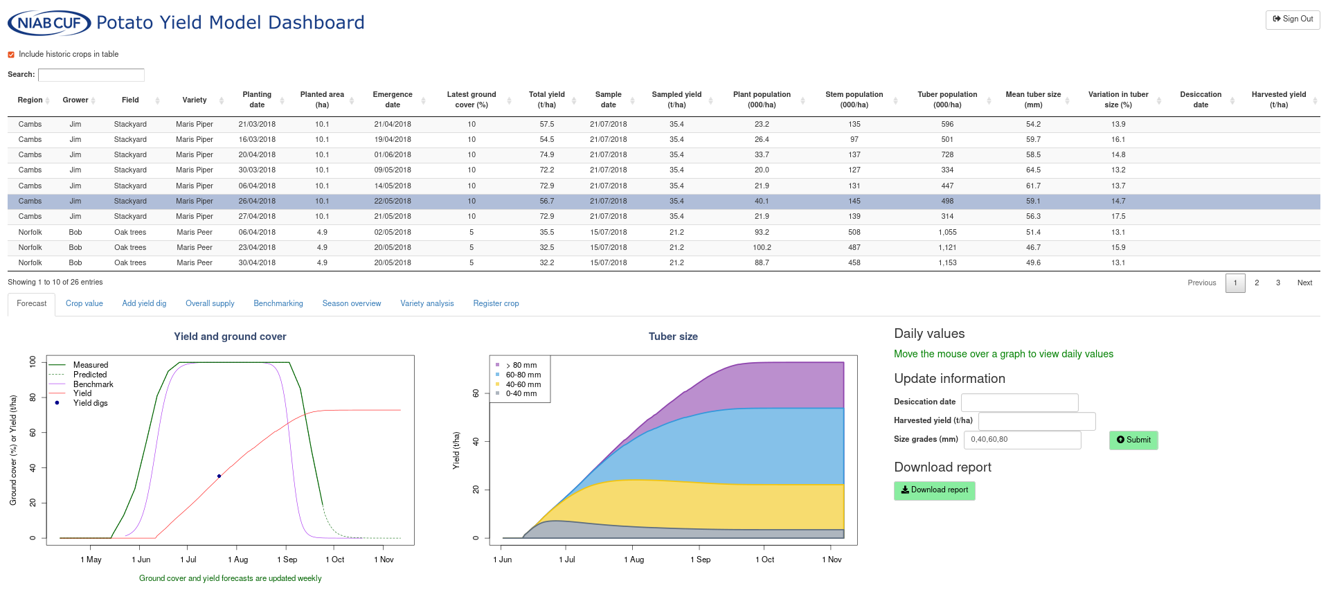
Potato Yield Model Dashboard

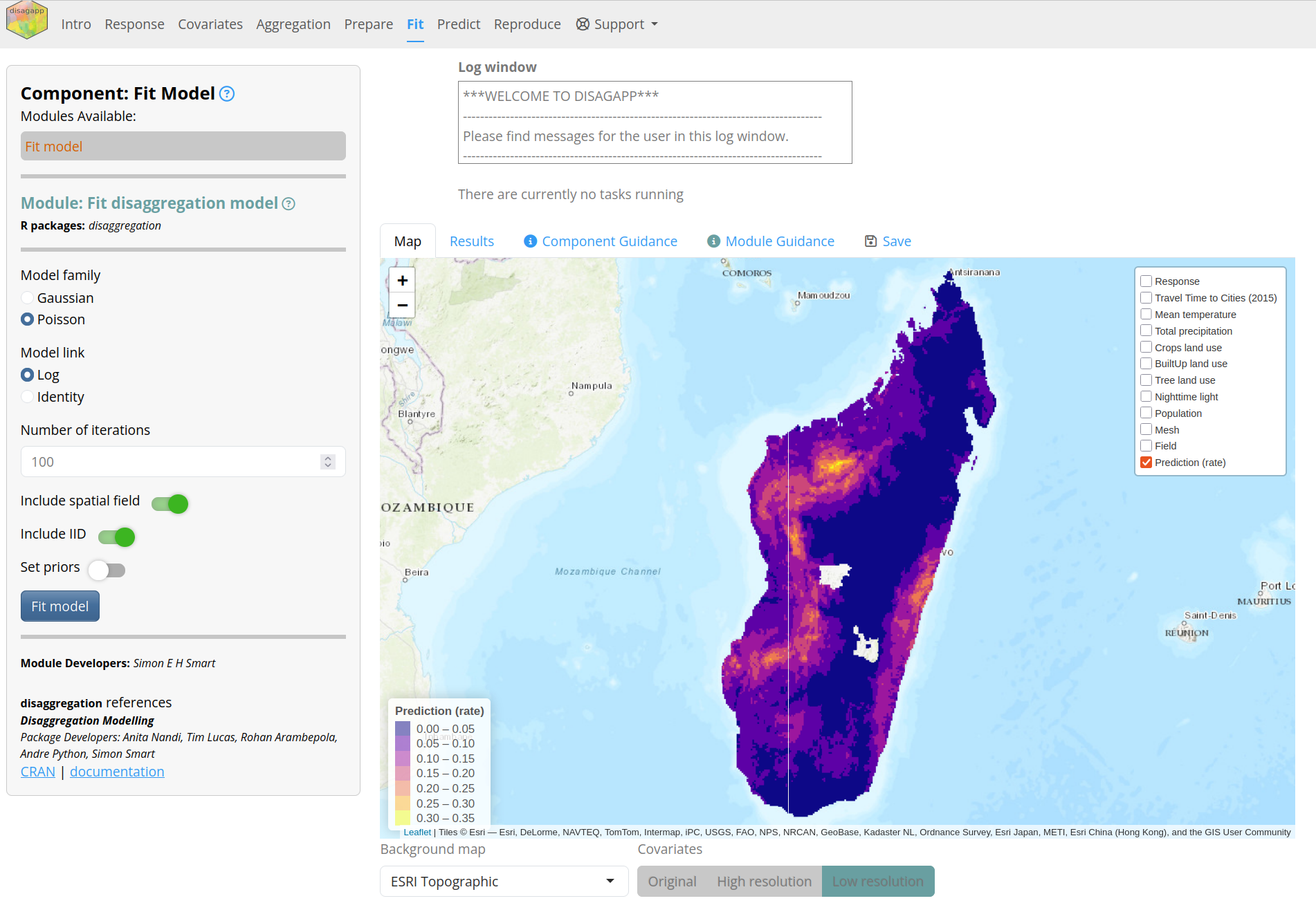
Disagapp simplifies disaggregation regression https://disagapp.le.ac.uk/

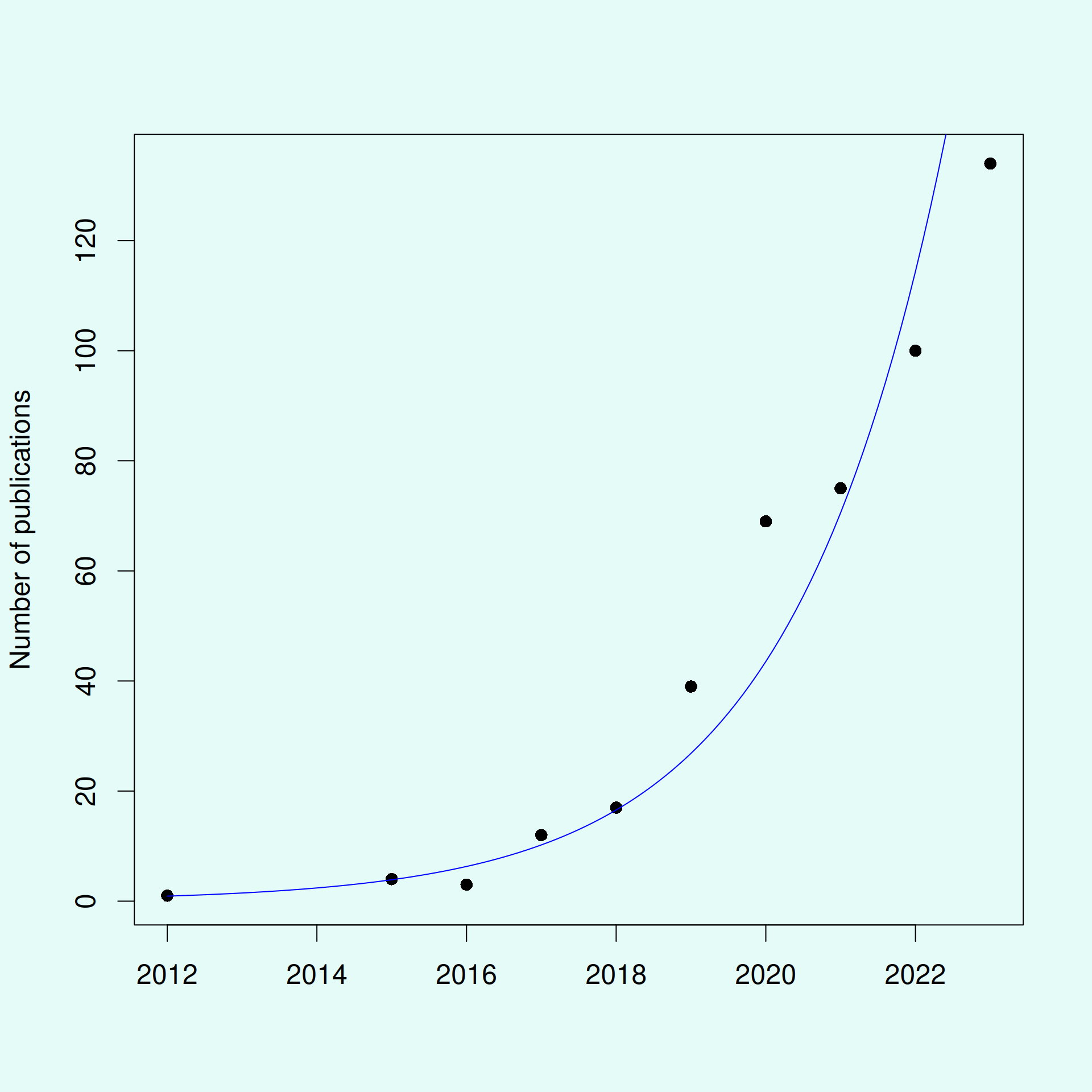
Shiny apps are becoming increasingly popular in academia

The low barrier to entry makes Shiny popular
Substantially increased apps as a method of dissemination
“shiny app” or “shiny application” in Web of Science:

The ease of development provides advantages and disadvantages

Simple apps can be created in an afternoon
Academics rarely have training in software development
What started simple can quickly snowball to become very complex

Data flows through an analysis in discrete steps

What characteristics should academic apps have?

Open

Attributable

Instructive

Reproducible

Reliable

Maintainable

There are many ways to structure shiny apps

50 apps published in 2023 were surveyed to determine current practices

The size and structure of codebases varied substantially

Other frameworks exist for making production quality shiny apps

{rhino} by Appsilon: dashboard-focused
{golem} by ThinkR: good but generic
{teal} by Insight Engineering / Roche: pharma-focused

`{shinymeta}` can also be used to create reproducible apps

Developed by Posit
Requires a lot of refactoring / unusual syntax
Unclear if it’s suited to large apps

server <- function(input, output) {
  var <- metaReactive({
    cars[[..(input$var)]]
  })
  output$Summary <- metaRender(renderPrint, {
    summary(..(var()))
  })
  output$code <- renderPrint({
    expandChain(output$Summary())
  })
}

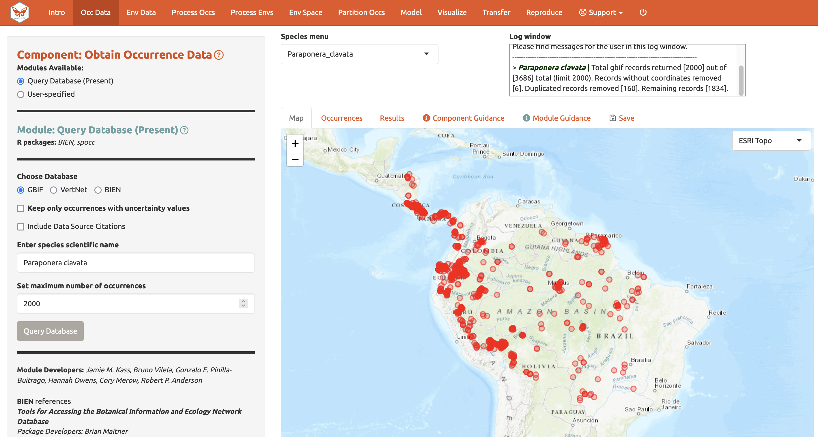
Wallace is an app for modelling species distributions

In development since 2015 with two major releases
Feature-rich with many ideal characteristics:

Error messages
Logging
Save and load

Reproducible
Cites packages used

Wallace provided the foundation to create shinyscholar

Lots of useful features that are difficult to implement from scratch
Removed all the modules
Adapted files so they could be edited programmatically

Various new features have been added since

Updated UI
Viewing source code
Running async tasks
End-to-end testing with {shinytest2}
Simplified reproducibility
Long-term reproducibility via {renv}
Automated tedious coding

Installation

install.packages("shinyscholar") installs all you need to create new apps
The package also includes an example app, which requires install.packages("shinyscholar", dependencies = TRUE) to run

Shinyscholar enforces a strict structure

Structured as a package
Analyses are split into components and modules
Each module calls a function
Each module is reproduced by a markdown chunk
Data is passed between modules through common

This structure has various advantages

Modules are self-contained
New modules slot in easily
Explicit for developers where code is located

Overview of the live demo

The package contains an example app
We’ll create a similar app and copy some of the modules
Then we’ll develop a new module and go through each of the steps to develop it

`create_template()` requires a dataframe of modules

component	long_component	module	long_module	map	result	rmd	save	download	async
select	Select data	async	Upload your own data	TRUE	FALSE	TRUE	TRUE	FALSE	TRUE
select	Select data	query	Query a database to obtain data	FALSE	FALSE	TRUE	TRUE	FALSE	FALSE
transform	Transform data	filter	Filter the data	TRUE	TRUE	TRUE	TRUE	TRUE	FALSE
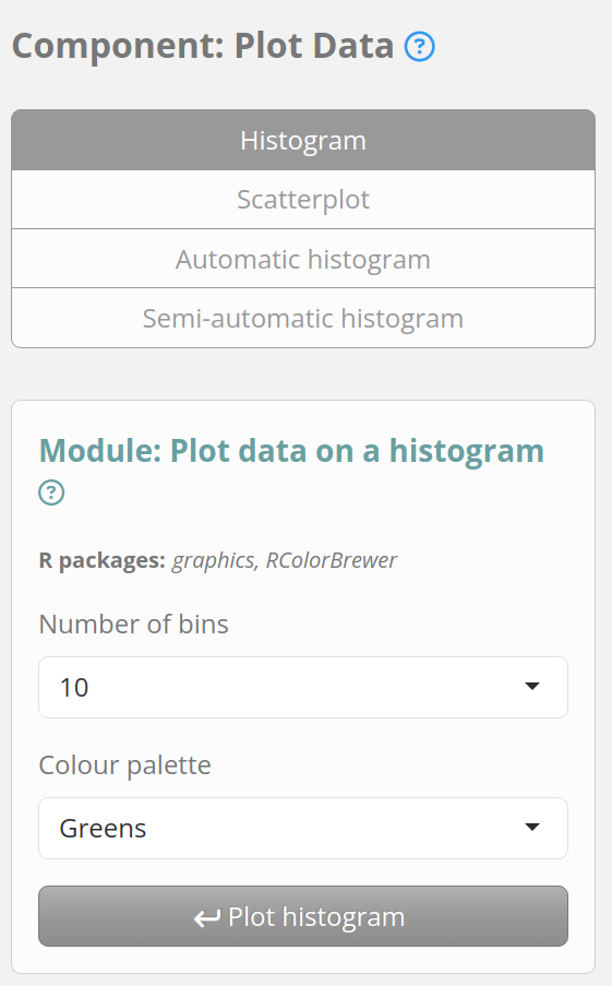
plot	Plot data	hist	Plot the data as a histogram	FALSE	TRUE	TRUE	TRUE	TRUE	FALSE
plot	Plot data	scatter	Plot the data as a scatterplot	FALSE	TRUE	TRUE	TRUE	TRUE	FALSE

Modules in disagapp

`common` is an object passed between modules

A shared environment for storing data
Avoids having to manually manage what data each module interacts with
Helps ensure consistent use of variable names
All set to NULL by default
common$reset() allows it to be reset

`common` in Disagapp

shape
response_name
agg
agg_prep
agg_prep_lores
covs

covs_prep
covs_prep_lores
covs_matrix
covs_summary
mesh
prep

fit
fit_plot
pred
transfer
map_layers
poly

`create_template()` creates an empty app 🚀

common_objects = c("raster", "histogram", "scatter")

shinyscholar::create_template(
  path = file.path("~", "Documents"), name = "SSdemo", author = "Simon Smart",
  include_map = TRUE, include_table = TRUE, include_code = TRUE, 
  common_objects = common_objects, modules = modules, install = TRUE)

SSdemo::run_SSdemo()

Structure of the app files

├── DESCRIPTION                                                 Define dependencies
├── inst
│   └── shiny
│       ├── common.R                                            Data objects shared between modules
│       ├── global.R                                            Loads package and modules
│       ├── ui_helpers.R                                        Functions to create module UI
│       ├── server.R                                            App server
│       ├── ui.R                                                App UI
│       ├── modules
│       │   ├── core_code.R                                     Displays code
│       │   ├── core_intro.R                                    Produces introductory walkthrough
│       │   ├── core_load.R                                     Loads app
│       │   ├── core_mapping.R                                  Creates map
│       │   ├── core_save.R                                     Saves app
│       │   ├── select_async.md                                 Module guidance
│       │   ├── select_async.R                                  Module UI and server
│       │   ├── select_async.Rmd                                Reproduces the module
│       │   ├── select_async.yml                                Module configuration
│       │   ├── ... (repeated for other modules)
│       ├── Rmd
│       │   ├── gtext_load.Rmd                                  Guidance text for each component
│       │   ├── gtext_plot.Rmd
│       │   ├── gtext_rep.Rmd
│       │   ├── references.Rmd                                  Template for rep_refPackages
│       │   ├── text_about.Rmd                                  Main panel on intro tab
│       │   ├── text_how_to_use.Rmd                             Detailed instructions
│       │   ├── text_intro_tab.Rmd                              Sidebar on intro tab
│       │   ├── text_loadsesh.Rmd                               Guidance for loading
│       │   ├── text_team.Rmd                                   Lists developers
│       │   ├── userReport_intro.Rmd                            Introduction to markdown
│       │   └── userReport_module.Rmd
│       └── www
│           ├── css
│           │   └── styles.css
│           ├── favicon.ico
│           ├── js
│           │   └── shinyjs-funcs.js
│           └── logo.png
├── R
│   ├── helper_functions.R                                      Various utility functions
│   ├── run_demo.R                                              Function to run app
│   ├── select_async_f.R                                        Function for each module
│   ├── select_query_f.R
│   ├── plot_histogram_f.R
│   └── plot_scatter_f.R
└── tests
    └── testthat
        ├── test-load_user.R                                    Tests for each module
        ├── test-load_database.R
        ├── test-plot_histogram.R
        └── test-plot_scatter.R

Shiny modules split code into manageable chunks

ui <- fluidPage(
  load_module_ui("load"),
  plot_module_ui("plot")
)

server <- function(input, output, session){
  load_module_server("load")
  plot_module_server("plot")
}

`input` and `output` IDs are namespaced

numericInput("number") 
plotOutput("plot") 

ns <- NS(id)
plotOutput(ns("plot"))
numericInput(ns("number"))

When used inside a module with an id of load, ns() appends load- to the ID so load-plot and load-number are created

By default though there is a lot to manage:

Sourcing the functions
Calling the functions
Passing data between modules
Reactivity between modules

Shinyscholar takes care of all of these!

Modules in shinyscholar have a broader definition and several files 🚀

In R/:
- Function: <component>_<module>_f.R
In inst/shiny/modules/:
- Shiny module: <component>_<module>.R
- Rmarkdown: <component>_<module>.Rmd
- Guidance: <component>_<module>.md
- Configuration: <component>_<module>.yml
In tests/:
- Tests: test-<component>_<module>.R

The logging system provides a flexible way to inform users

Messages can be sent to users via common$logger |> writeLog()
Either from inside the module function or the module server function

if (is.null(common$raster)) {
  common$logger |> writeLog(type = "error", "Please load a raster file")
  return()
}

The logging system provides a flexible way to inform users

When type = "info" / "warning" / "error" a shinyalert::shinyalert() modal is also displayed
type = "starting" / "complete" keep track of slow tasks
When logger = NULL inside a function, i.e. when used in the rmarkdown messages are passed to message(), warning() or stop() instead

Unusually, data is not reactive

Shiny is built to be reactive, but for large apps it can be difficult to control
Data in shinyscholar is not reactive
{gargoyle} is used instead to explicitly trigger reactivity

Gargoyle is used to trigger events

Each module’s identifier can be used to trigger events
init(<id>) is called during app start up
trigger(<id>) is called when a module runs successfully
watch(<id>) is used inside any outputs to be generated / other code that needs to run

Module development workflow

Data flow in shiny vs shinyscholar

flowchart TD
A[Input in UI] --> |input$| B([Computation in server])
B --> |output$| C(Output in UI)

class A sin
class B sser
class C sout

flowchart TD
A[Input in UI] --> |input$| C([Functions])
B[Existing data] --> |common$| C([Functions])
C --> |common$| D([Store in common])
D --> |output$| E(Output in Results)

class A sin
class B sin
class C sser
class D sser
class E sout

Developing the module function

Functions split the business logic from the shiny logic and enable reproducibility
First of all develop the function in an rmarkdown file
Once it works, move it to the function file and document
Parameters should either be common objects or input values

Functions should be written defensively

Check that inputs are correct and log any errors
May be not always be necessary when used in the app but we’re also creating user-facing functions used in the rmarkdown
Catch any other errors and fail gracefully instead of crashing the app

The `select_query()` function in the example app is most complex 🚀

select_query <- function(poly, date, token, logger = NULL) {

  check_suggests()

  if (!("matrix" %in% class(poly))){
    logger |> writeLog(type = "error","poly must be a matrix")
    return()
  }

  if (!is.character(date) || is.na(as.Date(date, format = "%Y-%m-%d"))) {
    logger |> writeLog(type = "error","date must be a string with the format YYYY-MM-DD")
    return()
  }

  if (nchar(token) < 200 || is.null(token)){
    logger |> writeLog(type = "error", "This function requires a NASA token - see the documentation")
    return()
  }

  # convert to terra object to calculate area and extent
  terra_poly <- terra::vect(poly, crs = "EPSG:4326", type = "polygons")
  area <- terra::expanse(terra_poly, unit = "km")
  if (area > 1000000) {
    logger |> writeLog(type = "error", paste0("Your selected area is too large (",round(area,0)," km2)",
                                              " when the maximum is 1m km2. Please select a smaller area"))
    return()
  }

  bbox <- c(min(poly[,1]), max(poly[,2]), max(poly[,1]), min(poly[,2]))

  search_url <- glue::glue("https://ladsweb.modaps.eosdis.nasa.gov/api/v2/content/archives?products=MCD15A2H&temporalRanges={date}&regions=[BBOX]W{bbox[1]}%20N{bbox[2]}%20E{bbox[3]}%20S{bbox[4]}&archiveSets=61")
  check <- check_url(search_url)

  if (!is.null(check)){
    image_req <- httr2::request(search_url ) |>
                  httr2::req_auth_bearer_token(token) |>
                  httr2::req_perform()

    image_resp <- image_req |> httr2::resp_body_html()

    image_links <- xml2::xml_find_all(image_resp, "//a")
    image_urls <- xml2::xml_attr(image_links, "href")
  } else {
    logger |> writeLog(type = "error", "The FAPAR API is currently offline")
    return()
  }

  # download and stitch together tiles
  raster <- NULL
  for (file in image_urls){
    if (tools::file_ext(file) == "hdf"){
      req <- httr2::request(file) |>
        httr2::req_auth_bearer_token(token) |>
        httr2::req_perform()

      temp <- tempfile(fileext = ".hdf")
      writeBin(httr2::resp_body_raw(req), temp)

      tile <- terra::rast(temp)$Fpar_500m
      if (is.null(raster)){
        raster <- tile
      } else {
        raster <- terra::merge(raster, tile)
      }
    }
  }

  if (is.null(raster)){
    logger |> writeLog(type = "error", paste0("No data was found for your selected area. ",
                                               "This could be due to cloud coverage or because the area is not over land."))
    return()
  }

  # reproject and crop
  raster <- terra::project(raster, "EPSG:4326")
  raster <- terra::crop(raster, terra_poly)

  # count missing values and log accordingly
  missing_values <- length(terra::values(raster)[terra::values(raster) > 1])
  urban <- length(terra::values(raster)[terra::values(raster) == 2.5])
  water <- length(terra::values(raster)[terra::values(raster) == 2.54])

  if (missing_values == terra::ncell(raster)) {
    logger |> writeLog(type = "error", paste0("No data was found for your selected area. ",
                                               "This could be due to cloud coverage or because the area is not over land."))
    return()
  }
  if (missing_values > 0) {
    message <- glue::glue("{missing_values} pixels were removed.")
    if (urban > 0) {
      message <- paste(message, glue::glue("{urban} pixels were removed due to urban land use."), sep = " ")
    }
    if (water > 0) {
      message <- paste(message, glue::glue("{water} pixels were removed due to water coverage."), sep = " ")
    }
    logger |> writeLog(message)
  }

  # remove missing values and rescale data to 0 - 100 %
  raster <- terra::clamp(raster, upper = 1, value = FALSE) * 100

  raster
}

Unit testing {.mediumcode} 🚀

Each module should have unit tests and end-to-end tests
Unit test tests that the module function behaves as you expect
End-to-end tests check that the whole module works

test_that("Check select_user function works as expected", {
  result <- select_user()
  expect_true(is.null(result))
})

The shiny module contains several functions

<identifier>_module_ui() - user inputs
<identifier>_module_server() - server function
Optionally:
<identifier>_module_result() - display outputs
<identifier>_module_map() - modify the map
<identifier>_module_rmd() - transfer data to rmarkdown

Only Input functions are included in the module UI

Input IDs need wrapping in ns()
Everything is wrapped in tagList

plot_hist_module_ui <- function(id) {
  ns <- NS(id)
  tagList(
    selectInput(ns("bins"), "Number of bins", choices = c(10, 20, 50, 100)),
    selectInput(ns("pal"), "Colour palette", choices = c("Greens", "YlOrRd", "Greys", "Blues")),
    actionButton(ns("run"), "Plot histogram")
  )
}

The server contains an `observeEvent()` triggered by `input$run`

Inputs are checked and any errors logged
Inputs are passed to the module function
Input values are stored in common$meta
Module function is called and results stored in common
Use trigger() to run anything that relies on the results
Use show_map() or show_results() to change the view

The server contains an `observeEvent()` triggered by `input$run`

  observeEvent(input$run, {
    # WARNING ####
    if (is.null(common$raster)) {
      common$logger |> writeLog(type = "error", "Please load a raster file")
      return()
    }
    # FUNCTION CALL ####
    raster_name <- c(common$meta$select_query$name, common$meta$select_async$name, common$meta$select_user$name)
    histogram <- plot_hist(common$raster, as.numeric(input$bins), input$pal, raster_name, common$logger)
    # LOAD INTO COMMON ####
    common$histogram <- histogram
    # METADATA ####
    common$meta$plot_hist$bins <- as.numeric(input$bins)
    common$meta$plot_hist$pal <- input$pal
    common$meta$plot_hist$name <- raster_name
    # TRIGGER ####
    trigger("plot_hist")
    show_results(parent_session)
    shinyjs::show("download")
  })

Outputs are triggered when the module runs successfully

output$hist <- renderPlot({
  watch("plot_hist")
  req(common$histogram)
  common$histogram()
  })

Outputs are inserted into the results tab {.mediumcode} 🚀

The visible results are determined by the module currently selected

plot_hist_module_result <- function(id) {
  ns <- NS(id)
  plotOutput(ns("hist"))
}

Saving and loading

When the app is saved, common is saved to an .Rds
Each module’s input values are stored in common$state
Distinct from those stored in common$meta which are only for modules that have been run

Saving and loading

Loading reloads data into common
Input values are restored from common$state
Module outputs are retriggered from names(common$meta)

The ability to save is also helpful during development

If working on a feature that relies on results from a slow step, it can be tedious to rerun each time a change is made
We can load common in outside shiny and use the exact data used in the app
Set load_file_path to point to a save file and it will be loaded automatically

`save_and_load()` takes care of tedious coding {.mediumcode} 🚀

Currently only default {shiny} inputs are supported

save_and_load(".") # for all modules
save_and_load(".", module = "component_module") # for a single module

numericInput(ns("number"), "Enter a number", value = 5)

list(number = input$number) # save
updateNumericInput(session, "number", state$number) # load

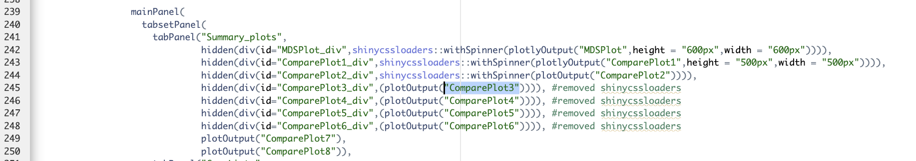
Markdown files can be merged to replicate the analysis

When a module is used an object becomes TRUE
Input values are stored and knitted into the markdown
Each chunk of the markdown calls the same function as the module in the app
The chunks for used modules are combined into one .Rmd file

Input values are copied into the rmarkdown

#```{r, echo = {{select_query_knit}}, include = {{select_query_knit}}}
poly <- {{select_query_poly}}
token <- {{select_query_token}}
ras <- select_query(poly, {{select_query_date}}, token)
raster_name <- {{select_query_name}}
#```

To create a reproducible chunk {.mediumcode} 🚀

#```{r}
poly <- structure(c(-0.871582, -0.871582, 0.322266, 0.322266, -0.871582, 
                    42.136253, 43.421009, 43.421009, 42.136253, 42.136253), 
                  dim = c(5L, 2L), dimnames = list(    NULL, c("longitude", "latitude")))
token <- NULL
raster <- select_query(poly, "2024-10-09", token)
raster_name <- "FAPAR"
#```

You can also add data directly to the markdown

If the output of a module is a small dataframe (~ 1000 values) then you can insert the common object straight into the markdown
Especially useful if files are uploaded as that can’t be reproduced automatically
Alternatively, download a .zip of data and load that in the markdown (example below)

As for saving and loading, `metadata()` takes care of some of the tedium 🚀

Unlike for save_and_load() this requires manual work afterwards and can therefore only be called once for each module

metadata(".") # for all modules
metadata(".", module = "component_module") # for a single module

numericInput(ns("number"), "Enter a number", value = 5)

common$meta$component_module$number <- input$number # store
component_module_number <- common$meta$component_module$number # transfer to Rmd
{{component_module_number}} # use in Rmd

End-to-end tests 🚀

test_that("{shinytest2} recording: e2e_select_user", {
  app <- shinytest2::AppDriver$new(app_dir = system.file("shiny", package = "demo"), name = "e2e_select_user")
  app$set_inputs(tabs = "select")
  app$set_inputs(selectSel = "select_user")
  app$click("select_user-run")
  common <- app$get_value(export = "common")
  expect_true(is.null(common$scatter))
})

Asynchronous modules

A major limitation of R and therefore Shiny is that it is single-threaded by default
When a slow operation is occurring apps become unresponsive to the user and anyone else connected to the same instance
ExtendedTask was added in Shiny v1.8.1 and enables tasks to run in the background

Slow running tasks can block the UI

Asynchronous modules

When async = TRUE for a module a different skeleton is used
The structure is different since starting the task and dealing with the results are separate
The number of currently running tasks is shown under the logger

The normal logger can’t be accessed from inside async tasks

asyncLog() is similar to writeLog() but can be used inside async functions
Use async = FALSE as the last parameter instead of logger = NULL
return(async %>% asyncLog("message)) sends errors back

  if (!is.character(date) || is.na(as.Date(date, format = "%Y-%m-%d"))) {
    return(async %>% asyncLog(type = "error", "date must be a string with the format YYYY-MM-DD"))
  }

We can listen for messages in the server and then pass to the logger

    if (class(result) == "list"){ # whatever the successful class is
      common$raster <- result
    } else {
      common$logger %>% writeLog(type = "error", result)
    }

Info and support

README at https://simon-smart88.github.io/shinyscholar/index.html
Bug reports and feature requests: https://github.com/simon-smart88/shinyscholar/issues
Any other questions: simon.smart@cantab.net

Acknowledgments

Tim Lucas for supervision
Wellcome for funding
Wallace developers

Shinyscholar

Overview

About me

Tomvision

Potato Yield Model Dashboard

Disagapp simplifies disaggregation regression https://disagapp.le.ac.uk/

Shiny apps are becoming increasingly popular in academia

The ease of development provides advantages and disadvantages

Data flows through an analysis in discrete steps

What characteristics should academic apps have?

There are many ways to structure shiny apps

There are many ways to structure shiny apps

There are many ways to structure shiny apps

50 apps published in 2023 were surveyed to determine current practices

The size and structure of codebases varied substantially

Other frameworks exist for making production quality shiny apps

{shinymeta} can also be used to create reproducible apps

Wallace is an app for modelling species distributions

Wallace is an app for modelling species distributions

Wallace provided the foundation to create shinyscholar

Various new features have been added since

Installation

Shinyscholar enforces a strict structure

This structure has various advantages

Overview of the live demo

create_template() requires a dataframe of modules

Modules in disagapp

common is an object passed between modules

common in Disagapp

create_template() creates an empty app 🚀

Structure of the app files

Shiny modules split code into manageable chunks

input and output IDs are namespaced

By default though there is a lot to manage:

Modules in shinyscholar have a broader definition and several files 🚀

The logging system provides a flexible way to inform users

The logging system provides a flexible way to inform users

Unusually, data is not reactive

Gargoyle is used to trigger events

Module development workflow

Data flow in shiny vs shinyscholar

Developing the module function

Functions should be written defensively

The select_query() function in the example app is most complex 🚀

Unit testing {.mediumcode} 🚀

The shiny module contains several functions

Only Input functions are included in the module UI

Input widgets are inserted to the sidebar

The server contains an observeEvent() triggered by input$run

The server contains an observeEvent() triggered by input$run

Outputs are triggered when the module runs successfully

Outputs are inserted into the results tab {.mediumcode} 🚀

Saving and loading

Saving and loading

The ability to save is also helpful during development

save_and_load() takes care of tedious coding {.mediumcode} 🚀

Markdown files can be merged to replicate the analysis

Input values are copied into the rmarkdown

To create a reproducible chunk {.mediumcode} 🚀

You can also add data directly to the markdown

As for saving and loading, metadata() takes care of some of the tedium 🚀

End-to-end tests 🚀

Asynchronous modules

Slow running tasks can block the UI

Asynchronous modules

The normal logger can’t be accessed from inside async tasks

We can listen for messages in the server and then pass to the logger

Info and support

Acknowledgments

`{shinymeta}` can also be used to create reproducible apps

`create_template()` requires a dataframe of modules

`common` is an object passed between modules

`common` in Disagapp

`create_template()` creates an empty app 🚀

`input` and `output` IDs are namespaced

The `select_query()` function in the example app is most complex 🚀

The server contains an `observeEvent()` triggered by `input$run`

The server contains an `observeEvent()` triggered by `input$run`

`save_and_load()` takes care of tedious coding {.mediumcode} 🚀

As for saving and loading, `metadata()` takes care of some of the tedium 🚀