Shiny workshop
Natural History Museum
Simon Smart
2024-02-07
About me
- Background in plant sciences and agricultural science
- Latecomer to R, only started in 2018
- Software developer in Population Health Sciences at University of Leicester with Tim Lucas
- Collaborating with Dave Redding on Disagapp for high-resolution mapping of disease
- https://github.com/simon-smart88
Workshop overview
- Trying to be broad but shallow so you know what’s possible, rather than narrow but exhaustive
- Please interrupt: If you’re not sure then someone else isn’t
- Aiming for 50:50 me talking:you writing
- Code examples are not always complete i.e. not all required arguments are used
- Natalie can help with Shiny, Tim with general R
Overview for this morning
- Introduction to Shiny
- Reactivity and why writing Shiny code differs from normal R
- Create example apps
Overview for the afternoon
- User interface design
- Interactive tables and maps
- Deploying your app to the web
- Common problems and debugging
What is Shiny?
- R package developed by Posit/Rstudio, first released in 2012
- Framework for developing interactive web apps using R
- No need to learn any web development (html, css, javascript)
- If you can do something in R, you can publish it online using Shiny
Download materials
git clone https://github.com/simon-smart88/shinyworkshop
install.packages(c("shiny","leaflet", "DT", "rsconnect", "sf", "terra"))- For the slides to be interactive, you need to run
slides.qmd
Structure of a Shiny app
Shiny apps consist of a user interface object (UI) and a server object
Structure of a Shiny app
Shiny apps consist of a user interface object (UI) and a server object
- Our job is to make these objects talk to each other
Communication between the UI and server
- The server function takes two
list()-like objects as arguments:input$where settings made in the UI are stored- Created for you by objects in the UI
- Values are read-only
output$where objects created in the server that need to be displayed in the UI are stored- You create them
flowchart TD
A[Input in UI] --> |input$| B([Computation in server])
B --> |output$| C(Output in UI)

class A sin
class B sser
class C sout
Input and output IDs
- The objects in
input$andoutput$have an ID used to refer to them - These must be unique or you will get errors
- For
input$objects, the ID is always the first argument of the function used to create them:
Input and output IDs
- For
output$objects, you declare them and then reference them by ID in the UI:
- Both are referenced as strings in the UI but as variables in the server
Reactivity basics
- Code in the server function is reactive
- If an
input$value changes, then any code which uses the input is rerun - Similarly, any code that uses a value calculated from the input is also rerun
- Unlike in a normal R script, code isn’t executed from top to bottom
flowchart TD
A[Input in UI] --> |input$| B([Computation in server])
B --> |output$| C(Output in UI)

class A sin
class B sser
class C sout
A simple example
flowchart TD
A["textInput()"] --> |input$name| B(["renderText()"])
B --> |output$name_out| C("textOutput()")

class A sin
class B sser
class C sout
Shiny input widgets
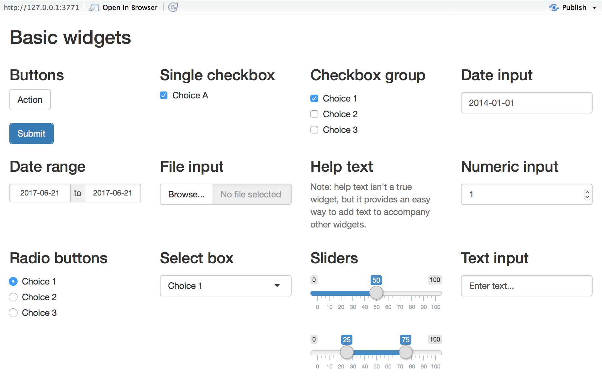
Source: https://shiny.posit.co/r/getstarted/shiny-basics/lesson3/
Output functions
Outputs are generated in the server using render* functions and displayed in the UI using *Output functions
| Data type | Render function | Output function |
|---|---|---|
| Table | renderTable() |
tableOutput() |
| Plot | renderPlot() |
plotOutput() |
| Text | renderText() |
textOutput() |
| Image | renderImage() |
imageOutput() |
| Interactive table | renderDataTable() |
dataTableOutput() |
Curly bracket syntax
- Typically
render*()functions are used with curly brackets{}inside the function - This lets you write multiple lines of code, but only the last line is returned
Another example
ui <- fluidPage(selectInput("animal", "Choose your favourite animal",
                            choices = c("","Whale", "Dinosaur")),
                textOutput("animal_name"))

server <- function(input, output) {
  output$animal_name <- renderText({
    animal_names = list("Whale" = "Hope", "Dinosaur" = "Dippy")
    paste0("Your favourite animal's name is ", animal_names[[input$animal]])})
}

shinyApp(ui = ui, server = server)UI development
- The UI object is one long list
fluidPage()makes the design responsive so that it fits on different sized screens- The first item will be placed in the top left
- Functions need separating by commas
Server development
- Shiny code is more complex to debug and errors may not be simple to understand
- Some mistakes won’t produce any errors at all
- First write code in an .Rmd file and then refactor for reactivity
- Start simple and build complexity gradually
- If you don’t already, use the F1 key to look at documentation
Static code can be put in different places
Static code can be put in different places
df <- read.csv()
# run once when the app starts

ui <- fluidPage()

server <- function(input, output) {

  df <- read.csv()
  # run whenever a new user uses the app

  output$table <- renderTable({
    df <- read.csv()
    # run whenever input$value changes
    df <- df[df$column == input$value,]
  })
}

shinyApp(ui = ui, server = server)
tidyverse peculiarities
Unfortunately this will not work as you might expect:
tidyverse peculiarities
- This is the correct syntax:
- See Mastering Shiny for more details
- For now, just use the old-fashioned method:
Exercise 1
- Create an app where you:
- Load data from
iris - Filter the data in some way using
sliderInput(),numericInput()orselectInput() - Display the filtered data using
renderTable()andtableOutput()
- Load data from
- Rstudio automatically detects
shinyApp()in a file and clicking on![]() will run the app
will run the app
 will run the app
reactive()
- If you want to access an
input$you must do so inside reactive objects - You have already done this - all the
render*functions are reactive - If you want to create an object without making an output though, you need to wrap it inside
reactive() - The resultant object is a function, so you need to append
()when you access the values
reactive() example
❌
✅
- Just like the
render*functions, you can make these multi-line using{}
File uploads
fileInput()uploads the file to the web server, but not into the R environment- The resulting
input$value is a dataframe containingname,size,typeanddatapathcolumns - To access the data, you need to process the file using the
datapathcolumn e.g.:
renderUI() and uiOutput()
- Used to generate UI elements containing values reliant on other inputs
observe()
- Similar to
reactive()but doesn’t return a result
Controlling reactivity
- Reactivity is essential for creating an interactive application but requires managing:
- What if some of your functions take seconds or minutes to run?
- What if your function uses an
input$which isNULLwhen the app initiates?
Using req()
req()is used to control execution of a function by defining the values that it requires- Placed at the top of reactive functions i.e.
reactive()andrender*() - If the conditions are not met, execution is halted
Using validate() and need()
validate(need())is similar toreq()but more user-friendly as errors can be passed back to the UI
Using actionButton() and bindEvent()
- Used to explicitly control when code is executed
Using actionButton() and observeEvent()
- Similar to using
bindEvent()but for use when the action doesn’t produce an output
Exercise 2
Create an app where you:
- Upload
iris.csvusingfileInput() - Select the names of two columns -
renderUI()andselectInput() - Plot the two columns in a scatter plot -
renderPlot() - Optional extra:
- Use
actionButtonandbindEvent()to control when the plot is rendered
- Use
flowchart TD
A["fileInput('file' ...)"] --> |input$file| B(["renderUI({<br/>selectInput(<br/>'variable_two' ...)<br/>})"])
A --> |input$file| C(["renderUI({<br/>selectInput(<br/>'variable_one' ...)<br/>})"])
B --> |output$select_two| D("uiOutput('select_two')")
C --> |output$select_one| E("uiOutput('select_one')")
E --> |input$variable_one|F
D --> |input$variable_two|F(["renderPlot()"])
F --> |output$plot|G("plotOutput('plot')")

class A sin
class B sser
class C sser
class D sout
class E sout
class F sser
class G sout
Downloads
downloadButton()in the UIdownloadHandler()in the server
Downloads
- Typically, you want to reuse a
reactive()that you have used to create a table or a graph inside thecontentpart of the download handler
df <- reactive(iris[iris$Sepal.Length <= input$sepal_length,])
output$plot <- renderPlot(plot(df()$Sepal.Length, df()$Sepal.Width))
output$download_data <- downloadHandler(
      filename = function() {
      "your_plot.png")
    },
    content = function(file) {
      png(file, width = 1000, height = 500)
      plot(df()$Sepal.Length, df()$Sepal.Width)
      dev.off()
    }
)
Interactive tables
- Datatables are created with
DT::renderDataTable()in the server andDT::dataTableOutput()in the UI: - For even fancier tables, check out
{reactable}and{gt}
Interactive tables
- You can access the selected row(s) using
input$<table ID>_rows_selected
Interactive maps
{leaflet}is a package for creating interactive mapsrenderLeaflet()for the server andleafletOutput()for the UI
An example
More leaflet
- Functions for:
- background maps -
addProviderTiles() - legends -
addLegend() - symbols -
addMarkers() - pop-ups -
addPopups() - zooming -
setView()andfitBounds() - controlling visible layers-
addLayersControl()
- background maps -
{leaflet.extras}has tools for drawing shapes on the map which can be used to edit data
Leaflet proxy
leafletProxy()prevents completely re-drawing the map whenever something changes:
Without leafletproxy
With leafletproxy
Accessing information from the map
- There are
input$values that record events occurring in the map input$<map ID>_<object type>_<event type>e.g.input$map_shape_click- The values are a
list()containing$latand$lngwhich can be used for further calculations - See the Inputs/Events section of https://rstudio.github.io/leaflet/shiny.html
output$selected_shape <- renderText({
  selected_point <- data.frame(x = input$map_shape_click$lng, y = input$map_shape_click$lat ) %>%
                     sf::st_as_sf(coords = c("x", "y"), crs = 4326)
index_of_polygon <- sf::st_intersects(selected_point, wards, sparse = T) %>%
                    as.numeric()
glue::glue("You clicked on the ward of {wards$NAME[index_of_polygon]} which is in {wards$DISTRICT[index_of_polygon]}")
  })
Accessing information from the map
Exercise 3
- Use
{leaflet}to select a ward or district of London and zoom when it is selected- Select the area either through clicking, or use a
selectInput() - Set the zoom using
sf::st_bbox()andleaflet::fitBounds()
- Select the area either through clicking, or use a
- Use a
downloadHandlerto download a.pngof the satellite imagery of just that area- Use
terra::crop(mask = TRUE)
- Use
UI layouts
- There are many different options for laying out the UI
- Sidebars, tabs, rows and columns
- Different components can be nested inside each other
- The examples in these pages need
layout.Rto be run separately (sorry!)
Sidebar layout
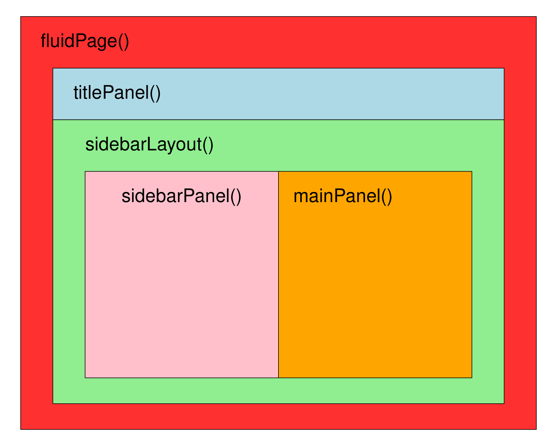
Sidebar layout
Tab panels
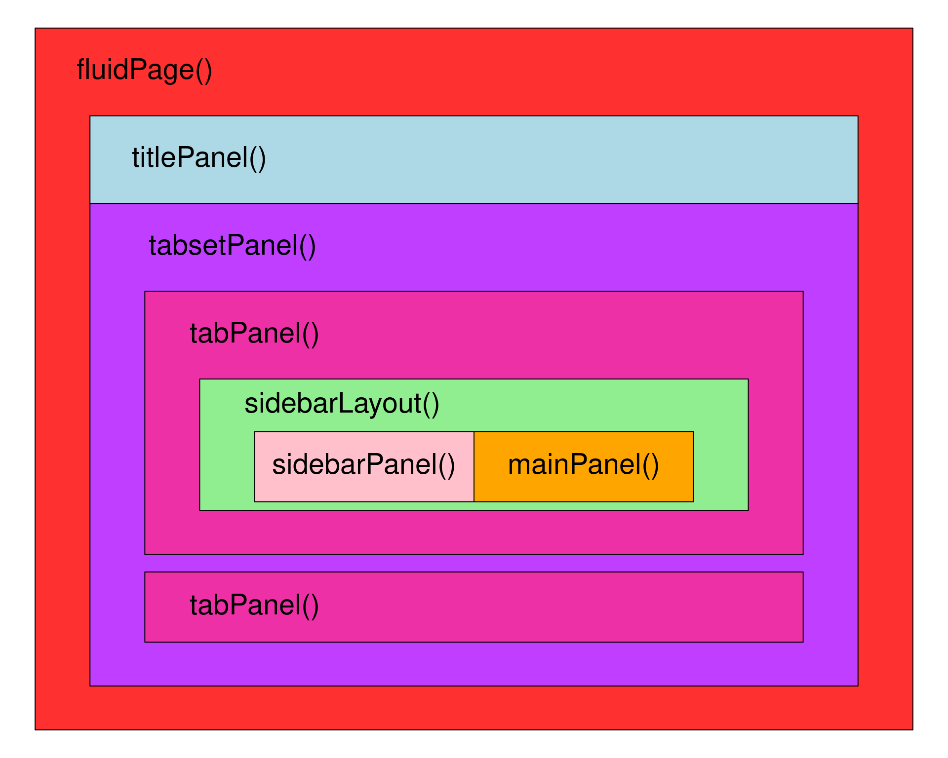
Tab panels
Fluid rows and columns
- Gives you more control over layout - the screen width is split into 12 units and you set their relative width
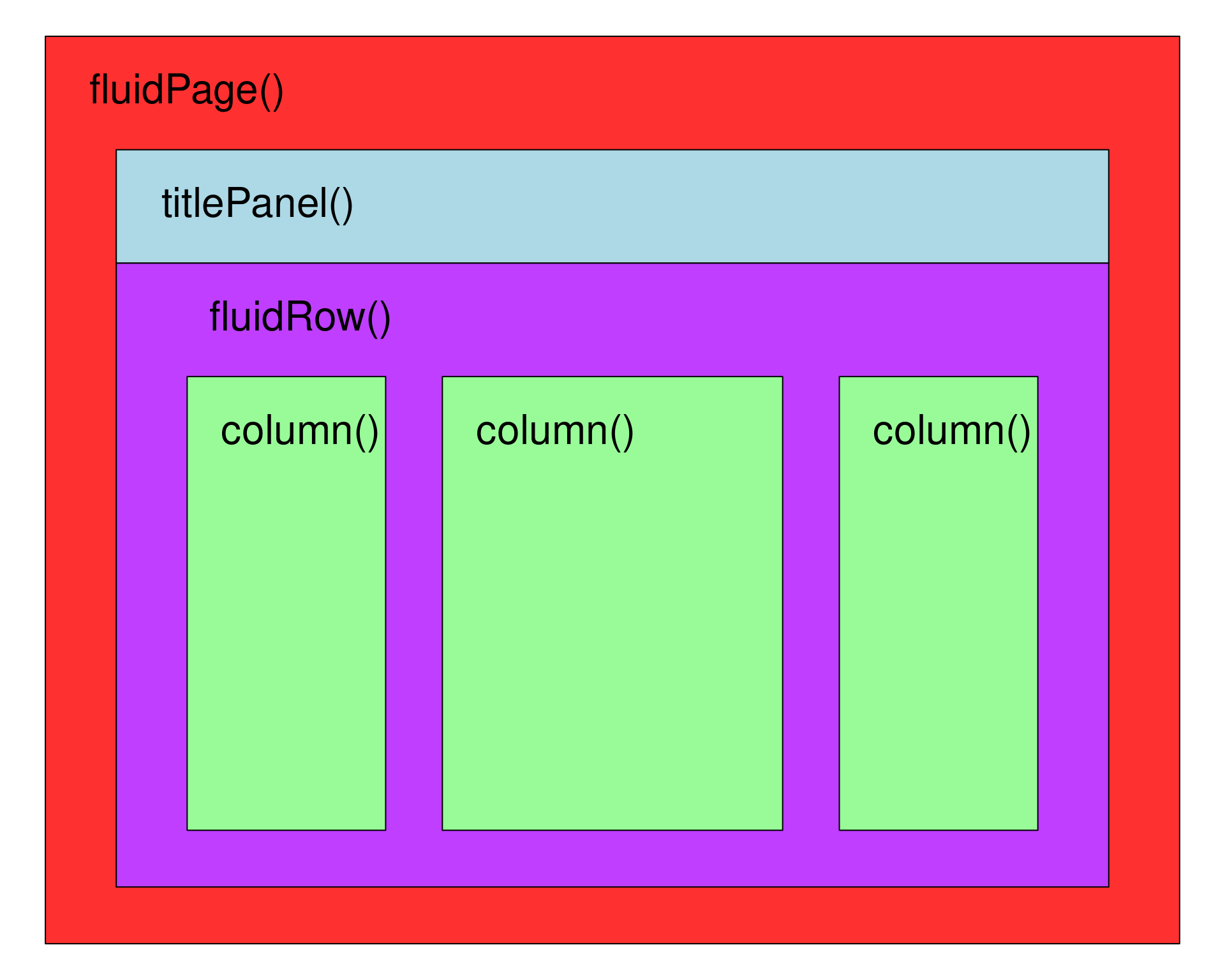
Fluid row and columns
Structuring UI code
Structuring UI code
- Brackets are important for structuring layout of elements
- Indentation and lines help to make your code readable
- It can get very complicated!
fluidPage(titlePanel("My fourth app"),
tabsetPanel(tabPanel("Tab 1",sidebarLayout(sidebarPanel(
numericInput("number", "Pick a number", value = 10),
selectInput("select", "Select an animal", choices = c("Cat", "Dog"))),
mainPanel(plotOutput("plot"),tableOutput("table")))),
tabPanel("Tab 2",fluidRow(column(width = 3,textInput("word", "Type a word"),
sliderInput("slider", "Pick a value", min = 10, max = 100, value = 50)),
column(width = 6,leafletOutput("map")),
column(width = 3,checkboxInput("check", "Tick me")))),
tabPanel("Tab 3",plotOutput("another_plot"))))
Structuring UI code
fluidPage(
  titlePanel("My fourth app"
  ),
  tabsetPanel(
    tabPanel("Tab 1",
      sidebarLayout(
        sidebarPanel(
          numericInput("number", "Pick a number", value = 10),
          selectInput("select", "Select an animal", choices = c("Cat", "Dog"))
        ),
        mainPanel(
          plotOutput("plot"),
          tableOutput("table")
        )
      )
    ),
    tabPanel("Tab 2",
      fluidRow(
        column(width = 3,
          textInput("word", "Type a word"),
          sliderInput("slider", "Pick a value", min = 10, max = 100, value = 50)
        ),
        column(width = 6,
          leafletOutput("map")
        ),
        column(width = 3,
           checkboxInput("check", "Tick me")
        )
      )
    ),
    tabPanel("Tab 3",
      plotOutput("another_plot")
    )
  )
)
Themes
- Themes can be used to change the appearance of all the elements of an app in one go
fluidPage(theme = bslib::bs_theme(bootswatch ="<theme name>"))- bootswatch.com
Cascading style sheets
- css determines the appearance of elements on web pages
- You can add your own css to the UI to change how elements appear
- Right-clicking / Ctrl+clicking allows you to inspect the html
- Often requires trial and error!
Exercise 4
- Add a UI layout and a theme the app you created in Exercise 3
- If time permits, add some more features:
- Name the file by the name of the ward/district
- Plot a histogram of the values of the ward
- A league table of greenness where clicking on a row zooms to the ward
- Anything else!
- Deploy the app to shinyapps.io (coming up!)
File naming conventions for deployment
- Various file structures can be used depending on complexity
- Standalone file as
app.R- what we will use - Separate files for server and UI -
server.Randui.R global.R- loaded beforeserver.Randui.Rso can be a good place to load data- If
server.Randui.Rbecome very long, code can be modularised into infinite files
Deployment
- Publish your app so that others can use it
- We will use shinyapps.io run by Posit
- Free and easy to use but has limitations:
- Only 1GB RAM on free tier which may not be enough to run models
- Limited amount of use per month (25 hours)
- Only 3-5 concurrent users
- No persistent data storage
- Many other options available - speak to IT
What happens when you deploy
- Copies the code from the app directory
- Uses
{renv}to check your R version and what package versions the app uses - Replicates the environment of your machine on their server
- R runs on their server and sends the results to the browser
How to deploy
- Register: https://www.shinyapps.io/auth/oauth/signup
- Your username will become part of the URL
- Copy your token and secret: https://www.shinyapps.io/admin/#/tokens
- Click “Show” on right hand side and then “Show secret”
- Copy and run the code which looks like this:
How to deploy
- Rename
exercise3.Rtoapp.R - Run the
app.Rin Rstudio - Click the “Publish” button in the top right corner
- Choose a URL for the app
- Click “Publish” again and wait
Applications vs. scripts
- Execution is circular, not linear
- You are creating a range of possibilities for your user
- Applications have users and users can break things
Applications vs. scripts
- Try and consider all the possible ways a user could interact with your app and manage them
- e.g. what happens if you write this, but a user uploads a
.jpeginstead of.csv?
Applications vs. scripts
- Adding extra arguments to functions and using
validate(need())can help:
Common pitfalls
- Trying to use reactive objects in a non-reactive context
- Not appending reactive objects with
()when accessing their values - Naming a
reactive()variable the same as a loaded function - Typos in
inputoroutputIDs - Using the same ID twice
- Misplaced brackets or commas in UI
Debugging
- Sooner or later you are going to run into a problem
- Apps are run in their own environment, so you can’t inspect objects in the Rstudio environment tab
- Run the code in a standard R script or .Rmd to check it works as you expect
- Use
verbatimTextOutput()andtextOutput()to display objects - are they in the state you expect? - Include
options(shiny.fullstacktrace = TRUE)in the server - Add
browser()above where your code is failing and then inspect the objects in your environment - Create a simple app containing only the problematic elements (i.e. a minimal, reproducible example)
Resources
Keep in touch
- Please send me links to your creations!
- I’m happy to help if you are really stuck
- ss1545@le.ac.uk